Chapter 5: How Do We Compare Biological Sequences?

You may be surprised, but sixty years ago, the word "programming" had nothing to do with computer programming, but instead referred to finding optimal programs, in the sense of finding a military schedule for logistics. In the 1950s, the inventor of dynamic programming, Richard Bellman, joined the RAND Corporation, which at the time was working on various contracts for the US Defense Department. At that time, the Secretary of Defense, Charles Wilson, was under pressure to reduce the military budget, including the research budget. Here is how Bellman described his interactions with Wilson and the birth of the term “dynamic programming”:

"[Wilson's] face would suffuse, he would turn red, and he would get violent if people used the term research in his presence. You can imagine how he felt, then, about the term mathematical… Hence, I felt I had to do something to shield Wilson and the Air Force from the fact that I was really doing mathematics inside the RAND Corporation. What title, what name, could I choose? In the first place I was interested in planning, in decision making, in thinking. But planning, is not a good word for various reasons. I decided therefore to use the word “programming”. I wanted to get across the idea that this was dynamic, this was multistage, this was time-varying I thought, lets kill two birds with one stone. Lets take a word that has an absolutely precise meaning, namely dynamic, in the classical physical sense. It also has a very interesting property as an adjective, and that is it's impossible to use the word dynamic in a pejorative sense. Try thinking of some combination that will possibly give it a pejorative meaning. It's impossible. Thus, I thought dynamic programming was a good name. It was something not even a Congressman could object to. So I used it as an umbrella for my activities."

Each recursive algorithm can be transformed into dynamic programming using a memoization technique that stores all results ever calculated by the recursive procedure in a table. When the recursive procedure calls an input which was already used, the results are just fetched from the table instead of launching a recursive call. However, memoization is only useful if your recursive algorithm arrives to the same situations many times, like in the case of RecursiveChange. For example, memoization becomes not very useful for algorithms like HanoiTowers since it is rarely called on the same input. Despite the fact that memoization does not immediately lead to an efficient non-recursive  algorithm for the Towers of Hanoi, such algorithms do exist (see https://www.geeksforgeeks.org/iterative-tower-of-hanoi/).

Yes, and below is some pseudocode.  Instead of making recursive calls, we simply embed the algorithm's iterations within a while loop.

IterativeOutputLCS(Backtrack, v, w)
    LCS ← an empty string
    i ← length of string
    j ← length of string w
    while i > 0 and j > 0
        if Backtrack(i, j) = "↓"
            i ← i-1
        else if Backtrack(i,j) = "→"
            j ← j-1
        else if Backtrack(i,j) = "↘"
              LCS ← concatenate vi with LCS
            i ← i-1
            j  ← j-1
    return LCS

All three types of backtracking edges (horizontal, vertical, and diagonal) are equally important; OutputLCS simply starts the analysis with vertical edges because it has to start somewhere! This will indeed bias the solutions if there are multiple longest common subsequences, in which case you may want to vary backtracking over multiple runs.

All topological orderings result in the same running time of your alignment algorithm, so you can choose any one you like.

Indel penalties are often implemented independent of the amino acid types in the inserted or deleted fragment, despite evidence that specific residue types are preferred in gap regions. For example, all indel penalties in the PAM matrix presented in the book are equal to 8, independently of which amino acid is inserted or deleted.

If we knew in advance where the conserved region between two strings begins and ends, then we could simply change the source and sink to be the starting and ending nodes of the conserved interval. However, the key point is that we do not know this information in advance. Fortunately, since local alignment adds free taxi rides from the source (0,0) to every node (and from every node to the sink (n, m)) of the alignment graph, it explores all possible starting and ending positions of conserved regions.

Unless biologists have a good reason to align entire strings (e.g., alignment of genes between very close species such as human and chimpanzee), they use local alignment.

Yes. For example, when biologists analyze the evolutionary history of a protein across various species, they often use global alignment. Also, most multiple alignment tools align entire sequences, rather than their substrings, as it is difficult to determine which substrings to align in the case of multiple proteins.

As mentioned in the text, an optimal local alignment fits within a sub-rectangle in the alignment graph. We denote the upper right and bottom left nodes of this sub-rectangle as (i, j) and (i’, j’), respectively.  Unless (i, j) = (0, 0) or (i’, j’) = (n, m), the local alignment corresponds to taking a free taxi ride (i.e., zero-weight edge) from (0, 0) to (i, j), taking one edge at a time to travel from  (i, j) to (i’, j’), and then taking another free taxi ride from (i’, j’) to (n, m).
We already know that (i’, j’) can be computed as a node such that the score s_{i’, j’} is maximized over all nodes of the entire alignment graph. The question, then, is how to backtrack from this node and to find  (i, j).

Recall the three backtracking choices from the OutputLCS pseudocode corresponding to the backtracking references ("↓",  "→", and "↘"). To these, we will simply add one additional option, "FREE", which is used when we have used a free taxi ride from the source and will allow us to jump back to (0, 0) when backtracking.  Thus, to find (i, j), one has to backtrack from (i’, j’) until we either reach a coordinate (i, j) with Backtrack_{i, j} = "FREE" or until we reach the source (0,0).

For simplicity, the following LocalAlignment pseudocode assumes that s_{i, j}  = -∞ if i < 0 or j < 0.

LocalAlignment(v, w, Score)
   for i ← 0 to |v|
      for j ← 0 to |w|
         si,j ← max{0, si-1,j + Score(vi, -), si,j-1 + Score(-, wj), si-1,j-1 + Score(vi, wj)}
         if si,j = 0
            Backtracki,j ← "FREE"
         else if si,j = si-1,j + Score(vi, -)
            Backtracki,j ← "↓"
         else if si,j = si,j-1 + Score(-, wj)
            Backtracki,j ← "→"
         else Backtracki,j ← "↘"
   return Backtrack

After computing backtracking references, we can compute the source node of the local alignment by invoking LocalAlignmentSource(Backtrack, i', j'), where (i', j') is the sink of the local alignment computed as a node with maximum score among all nodes in the alignment graph. The LocalAlignmentSource pseudocode is shown below.

LocalAlignmentSource(Backtrack, i, j)
   while i > 0 or j > 0
      if Backtrack(i, j) ="FREE"
         return (i, j)
      else if Backtrack(i, j) = "↓"
         i  ← i - 1
      else if Backtrack(i, j) = "→"
         j  ← j - 1
      else if Backtrack(i, j) = "↘"
         i  ← i - 1
         j  ← j - 1
   return (0,0)

Please take a look at the following figure for a big hint.

Indeed, selection of an appropriate PAM_n matrix is tricky, and biologists often use trial-and-error to select the most “reasonable” value of n when considering newly sequenced proteins. For this reason, they devised new BLOSUM matrices that are a bit easier to apply for protein comparison. See W.R. Pearson. Selecting the Right Similarity-Scoring Matrix, Current Protocols in Bioinformatics (2013).

The problem with this idea is that when computing the score at a node (i, j), we need to take into account the score of closing a gap from every node in the same row and same column. This is exactly what long indel edges do, and what we are trying to avoid in order to reduce the runtime of the algorithm by decreasing the number of edges in the graph.

For example, the figure below illustrates the two-level Manhattan for computing alignment with affine gap penalties (compare with the 3-level Manhattan shown in the text). At first glance, it looks like it solves the Alignment with Affine Gap Penalties Problem.

However, it you consider the following alignment with two gaps,

ATT--AA
A--GGAA

you will see that the path through the two-level graph for this alignment (shown below) miscalculates the alignment score; whereas the score of the alignment above is 3-2*(σ+ε), the score of the alignment in the figure below is 3- σ-3*ε.

Connecting (i, j)_middle to the nodes (i, j)_lower and (i, j)_upper (and assigning the edges a score of σ - ε) indeed seems like a more elegant approach to building a three-level Manhattan. However, in this case we would create directed cycles, since there would exist edges from (i, j)_lower and (i, j)_upper back to (i, j)_middle .

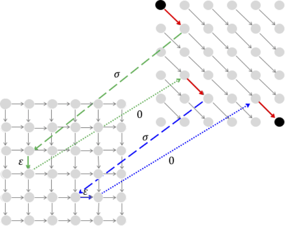
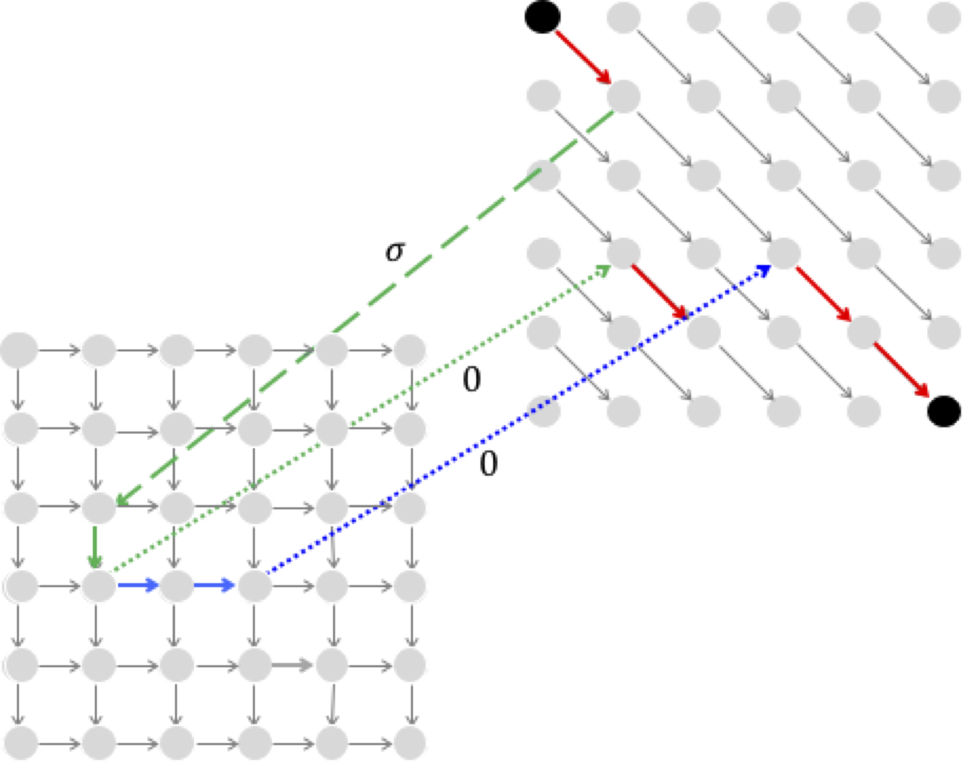
It appears that the alignment path in the one-level alignment graph shown below, which has a deletion of TT directly followed by an insertion of AA, is best represented by a sequence of edges that includes a direct edge from the lower level to the upper level.

However, such an edge is unnecessary because it can be represented by an edge from the lower to the middle level (weight 0) along with an edge from the middle to the upper level (weight -σ).

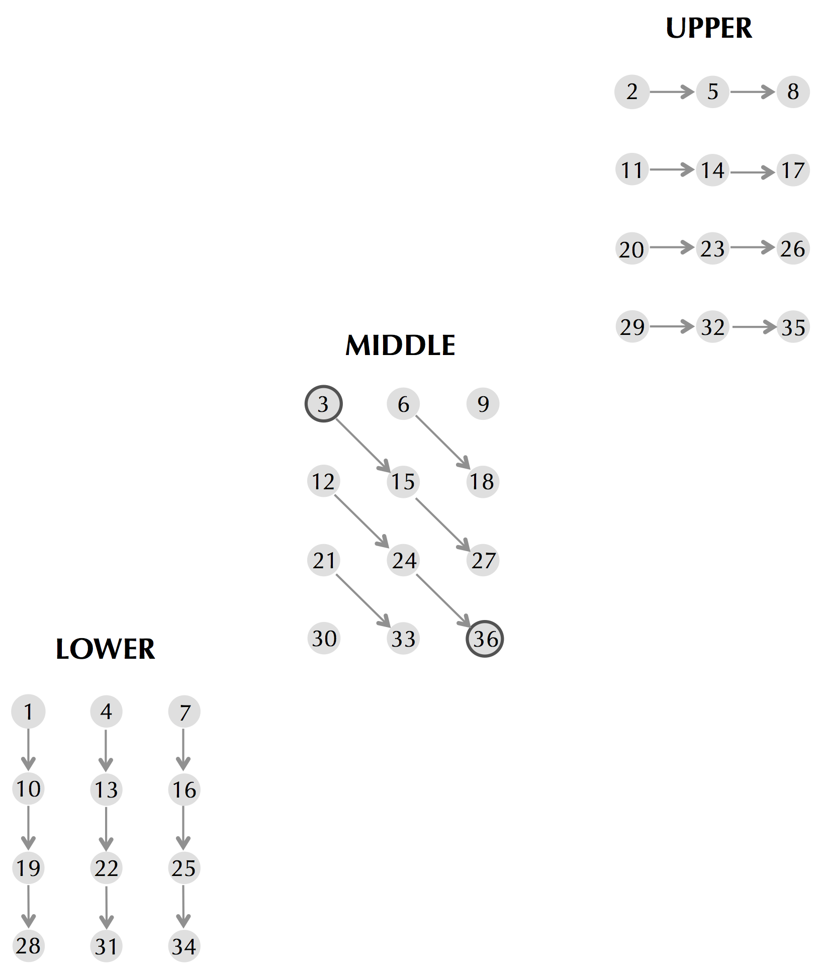
Please consult the following figure, which shows a topological order for a small three-level graph in which we proceed row-by-row in each level. (The topological order corresponds to visiting the nodes in increasing order, from 1 to 36.) Because there are some edges from (i, j)_lower to (i, j)_middle and from (i, j)_upper to (i, j)_middle for each i and j, we need to make sure that we visit (i, j)_lower and (i, j)_upper before (i, j)_middle.

Alignment with affine gap penalties is merely a search for a longest path in a DAG. Thus, backtracking in this graph is no different that backtracking in an arbitrary DAG, starting at the sink and proceeding toward the source according to a topological order. This reduces the problem to identifying a topological order, of which there are several.

It may be tricky to determine how to initialize the lower, upper, and middle matrices in the Alignment with Affine Gap Penalties Problem. For this reason, it may be easier to construct a DAG for this problem, approaching it as a general Longest Path in a DAG problem. Since we are interested in paths that start at the node (0,0) in the middle graph, we initialize this node with score 0. However, it is not the only node lacking incoming edges in the three-level graph for the Alignment with Affine Gap Penalties Problem, since the two other nodes lower_0,0 and upper_0,0 have this property as well. We therefore will initialize these two nodes with score -∞, since valid paths in the alignment graph must start at middle_0,0.

Note also that the recurrence relationships for the the Alignment with Affine Gap Penalties Problem include negative indices. For example, we must compute middle_i,-1 before computing middle_i,o. We therefore will also set the values of all variables with negative indices to -∞.

If the array Length(i) has more than one element of maximum value, then you can choose any of them, breaking ties arbitrarily.

It is also possible for a single longest path to have multiple middle nodes. This occurs if such a path has a vertical edge right after reaching the middle column (i.e., a path that traverses one or more edges in the middle column).

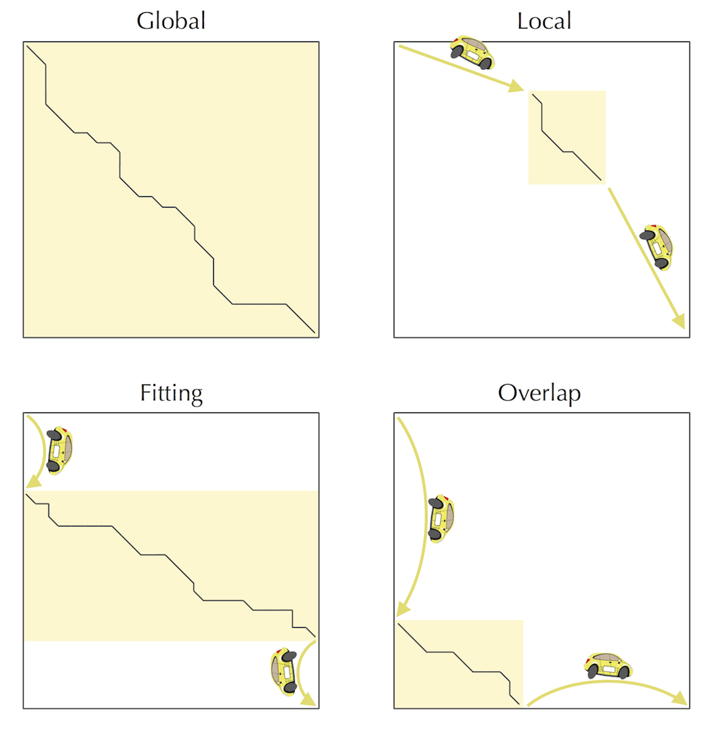
The shaded parts of the alignment graph to the northwest and southeast of the middle node make up more than half of the total area of the alignment graph. In contrast, the shaded parts of the alignment graph to the northwest and southeast of the middle edge make up less than half of the total area of the alignment graph. This implies that when we divide and conquer based on the middle node, we obtain runtime greater than 2nm, whereas when we divide and conquer based on the middle edge, we obtain runtime less than 2nm.

Although it may appear that switching from finding a middle node to finding a middle edge results in only a small speed-up and does not affect the asymptotic O(nm) estimate of the running time, it allows us to eliminate some annoying corner cases and simplify the pseudocode.

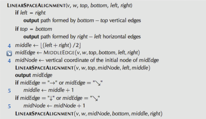
Below we illustrate how LinearSpaceAlignment works in the case top = 0, bottom = 8, left = 0, right = 8 shown below:

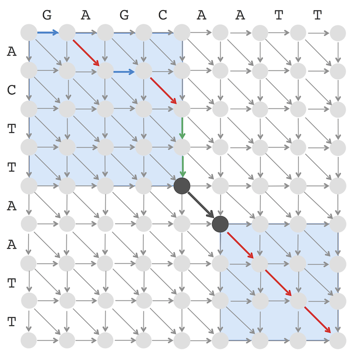
The numbers below in blue illustrate how variables change during the execution of LinearSpaceAlignment and result in two recursive calls LinearSpaceAlignment(v, w, 0, 4, 0, 4) and LinearSpaceAlignment(v, w, 5, 8, 5, 8) illustrated by two blue rectangles above. In the case when midEdge is horizontal or diagonal, the left blue rectangle is shifted by one column to the right as compared to the middle column (the line middle ← middle + 1). In the case when midEdge is vertical or diagonal, the left blue rectangle is shifted by one row to the bottom as compared to the position of the middle node (the line midNode ← midNode+1).

It is possible to extend our idea from pariwise alignment (in order to find a longest common subsequence) to more complex scoring models, e.g., for alignment with affine gap penalties. The only question is where to place the "middle column". It turns out that we need to consider two middle columns to implement the divide-and-conquer linear-space algorithm for alignment with affine gap penalties; try to figure out which ones!

Every alignment of a string v against a profile Profile = (P_{X, j}) (for X ∈ {A, C, G, T}, and 1 ≤ j ≤ m) can be represented as a path from (0,0) to (n, m) in the alignment graph. We can define scores of vertical and horizontal edges in this graph as before, i.e., by assigning penalties sigma to indels. There are various ways to assign scores to diagonal edges, e.g, a diagonal edge into a node (i, j) can be assigned a score P_{vi, j}. After the scores of all edges are specified, an optimal alignment between a string and a profile is computed as a longest path in the alignment graph.