
Chapter 2: Which DNA Patterns Play the Role of Molecular Clocks?
(Week 3)
Recent studies of Arabidopsis thaliana (a model organism for plant biology) have revealed that the circadian clock works differently than was described in our book and in Harmer et al., 2000. However, one of our learners, Bahar Behsaz, brought to our attention a recent article, Pokhilko et al., 2012. According to this article, the expression of CCA1 and LHY peaks in the early morning, whereas the expression of TOC1 peaks in the early evening. The authors showed that TOC1 in fact serves as a repressor of CCA1 and LHY in the morning loop.
Their revised circadian cycle is shown below (bottom left is the new version, upper right is the previous outline of the cycle).

Although GGGGA indeed represents the most conserved part of the NF-χB motif, the remaining seven less conserved positions do contribute to distinguishing real occurrences of the NF-χB binding sites from other sporadic 12-mers that contain GGGGA.
Since biologists do not know in advance the length of the regulatory motif, they try various values of k and select a solution that makes more sense. For example, if k is larger than the length of the regulatory motif, then the initial/ending positions in the computed motif will have low information content, implying that a smaller value of k makes more sense.
Most of these similar 15-mers result from spurious similarities and have nothing to do with the real implanted motifs. Thus, if we attempt to extend these spurious pairwise similarities in ten similar 15-mers (there are ten sequences in the Subtle Motif Problem), then we will fail.
Imagine three urns, each of which contains eight colored balls. The first urn contains eight balls of eight different colors. The second urn contains four blue balls, three green balls, and one red balls. The third urn contains eight blue balls. If you randomly draw a ball from an urn, then you are most certain about the outcome when drawing from the third urn, and the least certain about the outcome when drawing from the first urn. But can we somehow quantify this uncertainty?
In 1948, Claude Shannon (the founder of information theory) wanted to find a function H(p1, ... , pN) measuring the uncertainty of a probability distribution (p1, ... , pN). First, note that drawing balls from each urn can be represented as a probability distribution (i.e., a collection of nonnegative numbers summing to 1). For example, the respective probability distributions for the three urns are (1/8, 1/8, 1/8, 1/8, 1/8, 1/8, 1/8, 1/8); (4/8, 3/8,1/8); and (1).
Shannon made an important observation that we will illustrate using the urn example. Imagine that a red-green color-blind man draws a ball from the second urn. If he draws a blue ball, then he will immediately know it is blue, but he will not be able to distinguish between red balls and green balls. However, we can devise an equivalent experiment involving two draws. The color-blind man first draws a ball from an urn containing four blue and four black balls (the probability distribution is (1/2, 1/2)); then, if a black ball is chosen (with probability equal to 1/2), he then draws a ball from a separate urn containing three green balls and one red ball, marked "G" and "R" respectively so that he can distinguish them (again, the associated probability distribution is (3/4, 1/4)).
Although we have substituted a one-draw experiment with a two-draw experiment, Shannon's critical observation was that the uncertainty of the process should not have changed! In other words, the entropy of the first experiment (H(4/8, 3/8, 1/8)) should be equal to the entropy of the first draw (H(1/2, 1/2)) plus 1/2 times the entropy of the second draw (H(3/4, 1/4)), since there is probability 1/2 that the second draw will occur. Thus,
Shannon further argued that H should be a continuous function of (p1, ... pN), and that it should be maximized in the case of maximum uncertainty, which occurs when p1 = ... = pN = 1/N. It turns out that the only way H(p1, ... pN) can satisfy these conditions is if it is proportional to
and thus entropy was born.
In practice, information content is computed as H(p1, p2, p3, p4) + en, where en is a small-sample correction for a column of n letters. Small-sample correction is responsible for the height of G in the third and fourth position (see figure below reproduced from the text) being smaller than 2.
![]()
Please continue reading to the subsection "Why have we reformulated the motif finding problem?" to find out!
There are indeed four different notions of distance in this section. To make matters worse, we use the notation d(*, *) to refer to three of them -- the exception being Hamming distance.However, we see this not as a bug but as a feature, since we want you to think about these four notions of distance in the same framework because they are all related to each other. To determine what specific notion of distance we are talking about at any given point in time, you should pay attention to the arguments in d(*, *). Here are the four possible arguments for these cases:
- HammingDistance(k-mer, k-mer)
- d(k-mer, collection of k-mers)
- d(k-mer, string) -- where the string's length is at least equal to k
- d(k-mer, collection of strings) -- where each string's length is at least equal to k
To test your knowledge of these functions, first say that Pattern = ACGT and Pattern' = ATAT. Then HammingDistance(Pattern, Pattern') = 2. Second, say that Motifs = {TACG, GCGT, GGGG}. Then the Hamming distances between Pattern and each of these 4-mers are 4, 1, and 3 respectively; thus, d(Pattern, Motifs) = 4 + 1 + 3 = 8. Third, say that Text = TTACCATGTA. We know that d(Pattern, Text) is equal to the minimum Hamming distance between Pattern and any k-mer substring of Text. This Hamming distance is minimized by the substring ATGT of Text, so d(Pattern, Text) in this case is equal to 1. Finally, say that Dna = {AGACCAGC, ACGTT, CACCCATGTCGG}. In this case, d(Pattern, Dna) is equal to the sum of distances
The purpose of setting a variable equal to infinity is when initializing a variable x that you aim to minimize. The idea is to pick a number that is far larger than x could possibly be. If you want to get fancy, then initialize x to be the largest integer that can be encoded by your programming language.
Sure! Below is an example, and you may also like to read this blog post by our student Graeme Benstead-Hume. Consider the following matrix Dna, and let us walk through GreedyMotifSearch(Dna, 4, 5) when we select the 4-mer ACCT from the first sequence in Dna as the first 4-mer in the growing collection Motifs.
Although GreedyMotifSearch(Dna, 4, 5) will analyze all possible 4-mers from the first sequence, we limit our analysis to a single 4-mer ACCT:
TTACCTTAAC
AGGATCTGTC
Dna CCGACGTTAG
CAGCAAGGTG
CACCTGAGCT
We first construct the matrix Profile(Motifs) of the chosen 4-mer ACCT:
Motifs A C C T
A: 1 0 0 0
C: 0 1 1 0
Profile(Motifs) G: 0 0 0 0
T: 0 0 0 1
Since Pr(Pattern|Profile) = 0 for all 4-mers in the second sequence in Dna, we select its first 4-mer AGGA as the Profile-most probable 4-mer, resulting in the following matrices Motifs and Profile:
Motifs A C C T
A G G A
A: 1 0 0 1/2
C: 0 1/2 1/2 0
Profile(Motifs) G: 0 1/2 1/2 0
T: 0 0 0 1/2
We now compute the probabilities of every 4-mer in the third sequence in Dna based on this profile. The only 4-mer with nonzero probability in the third sequence is ACGT, and so we add it to the growing set of 4-mers:
A C C T
Motifs A G G A
A C G T
A: 1 0 0 1/3
C: 0 2/3 1/3 0
Profile(Motifs) G: 0 1/3 2/3 0
T: 0 0 0 2/3
We now compute the probabilities of every 4-mer in the fourth sequence in Dna based on this profile and find that AGGT is the most probable 4-mer:
CAGC AGCA GCAA CAAG AAGG AGGT GGTG
0 1/27 0 0 0 4/27 0
After adding AGGT to the matrix Motifs, we obtain the following motif and profile matrices:
A C C T
Motifs A G G A
A C G T
A G G T
A: 1 0 0 1/4
C: 0 2/4 1/4 0
Profile(Motifs) G: 0 2/4 3/4 0
T: 0 0 0 3/4
We now compute the probabilities of every 4-mer in the fifth sequence in Dna based on this profile and find that AGCT is the most probable 4-mer:
CACC ACCT CCTG CTGA TGAT GAGT AGCT
0 6/64 0 0 0 0 18/64
After adding AGCT to the motif matrix, we obtain the following motif matrix with consensus AGGT:
A C C T
A G G A
Motifs A C G T
A G G T
A G C T
You can select any set of k-mers to form the initial motif matrix BestMotifs. Note that as soon as a better collection of motifs are found, BestMotifs will be updated to this other collection.
Yes, the profile matrix with added pseudocounts may differ or even overestimate from the real probability distribution. But it presents the lesser of two evils, since we get ourselves into even bigger trouble if we don’t use pseudocounts. Furthermore, as another FAQ indicates, using a pseudocount value of 1 is not unreasonable in practice.
The choice of this parameter is arbitrary. However, perhaps surprisingly, changing the exact pseudocount value from 1 to 0.1 (or even to 0.00001) is unlikely to significantly change the results of the algorithms you implemented in this chapter. However, as described by Nishida et al., 2009, some caution is needed when selecting pseudocounts. These authors found that a good default pseudocount value is 0.8.
The performance of GreedyMotifSearch does in fact deteriorate when the first string in Dna does not contain k-mers similar to the consensus motif. For this reason, biologists often run GreedyMotifSearch multiple times, shuffling the strings in Dna each time.
(Week 4)
The common example of a Las Vegas algorithm is quicksort: https://en.wikipedia.org/wiki/Quicksort
A tetrahedron, as shown below.

In order to make your life easier. However, modifying RandomizedMotifSearch to add pseudocounts will improve its performance.
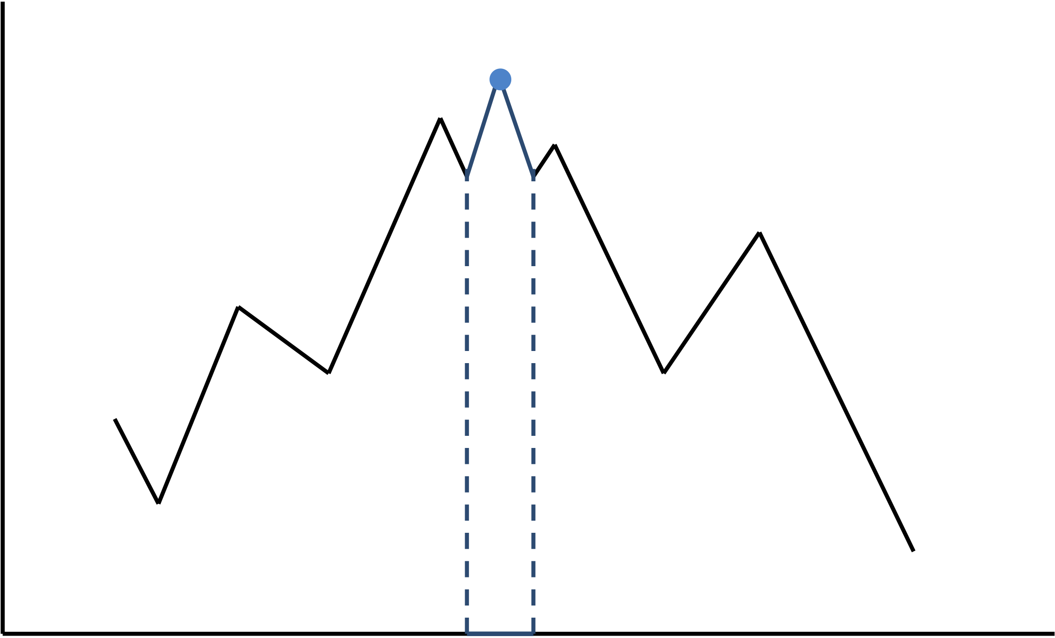
Consider the "mountain range" shown below, and imagine that the x-axis represents all possible motifs, while the y-axis represents their inverted score; that is, better motifs will have lower scores but higher inverted score. To find the lowest-scoring motif, we need to climb to the top of the tallest peak (shown by the blue point). If you are not willing to "climb down" sometimes, the only way you can reach the top is if your initially chosen motif corresponds to the short interval highlighted in blue, a low probability event. An example of an algorithm that is unwilling to "climb down" is if we select the most probable k-mer instead of selecting a Profile-randomly generated k-mer each time.
In many practical instances of motif finding, this probability may be less than one in a million, so that even if we repeat our search 1,000 times, starting with a randomly selected collection of k-mers each time, we will probably not reach the tallest peak. In these cases, it makes sense to design an algorithm that is allowed to climb down, thus potentially increasing the time required to make it to the top, but also increasing the probability of success despite a poor initial choice of motifs.
Even when GibbsSampler finds the correct motif before the end of the run, it remains unclear whether an even better scoring motif exists. As a result, it is unclear under what conditions GibbsSampler should be stopped. Biologists often run GibbsSampler a fixed number of times or until the score of the identified motif does not significantly improve after a large number of iterations.
It may seem counterintuitive yet also only slightly slows us down while keeping our algorithm easy to state.
There are no rigorous rules on how many times to run randomized algorithms other than "run them as many times as is feasible". In practice, researchers often allocate a certain computational resource (say, one hour of computing time) and make sure that a randomized algorithm completes within this fixed time interval. For example, if each run of RandomizedMotifSearch is 50 times faster than a run of GibbsSampler, then they can afford to run 50 times as many trials of RandomizedMotifSearch.
Genomes often have homonucleotide runs such as AAAAAAAAA and other low-complexity regions like ACACAACCA. When a homonucleotide run appears in each sequence in Dna, it will likely score higher than the real regulatory motif. For this reason, in practice, motif finding algorithms mask out low-complexity regions before searching for regulatory motifs.
ISBN: 978-0-9903746-3-3