Chapter 1: Where in the Genome Does DNA Replication Begin?

Sure! We wrote an appendix on pseudocode for readers wanting more background on the subject. Click here to download.

One of our first students on Coursera was Dr. Mate Ravasz, a biologist who was working on replication. The following answer is inspired by his response on the class discussion forum.

Knowing the origin of replication enables detailed studies of replication initiation. DNA replication requires various proteins to bind to ori, and once the replication machinery is ready, it activates itself and starts copying DNA. We know some but not all of the proteins involved in this process, and we still don't fully understand how these proteins contribute to replication. In fact, we have tried to hide the rather complicated details of the replication machinery, but you can check out the Prokaryotic DNA Replication page on Wikipedia to learn more.

An error during replication can lead to various diseases, including cancer. To understand how replication initiation works and what causes it to malfunction, we must first know where to look for replication origins. For this reason, we must accurately locate ori sites in the genome to study their replication initiation. Things are made even more difficult when we move from bacteria to more complex organisms; the human genome has thousands of origins of replication.

As mentioned in the main text, biologists often design self-replicating DNA segments, called plasmids, by inserting an origin of replication into them. This is a crucial capability for many genetic engineering experiments, since placing a plasmid into a cell will allow it to replicate. When a cell replicates, its plasmids are distributed to sister cells. Therefore, if we know more about replication origins, we can introduce foreign DNA into an organism and have it stably maintained.

DnaA does not necessarily bind to just one DnaA box. In fact, it may bind to all of them.

It is not immediately clear in Figure 1.3, reproduced below, whether observing three 9-mers in the replication origin of Vibrio cholerae is more surprising than observing four 8-mers or five 7-mers. See DETOUR: Probabilities of Patterns in a String for a discussion of how to select the value of k that results in the "most surprising" frequent k-mer.

Depending on the application, biologists may choose to analyze overlapping or non-overlapping k-mers. In the case when we search for DnaA boxes, this distinction is not very important, and we ask you to analyze overlapping k-mers because it makes the algorithms a bit easier to implement.

A Teaching Assistant in the first session of our Coursera class, Robin Betz (who is now a biophysics graduate student at Stanford University) responded to various questions on the Coursera discussion board. The following answer (along with some others) is motivated by one of her posts.

Mutations are the driving force of evolution in all domains of life, and no cell is immune to them. Moreover, mutations that arise in a child but are not present in either parent may lead to a disease. On average, humans acquire about 100 new mutations (called single nucleotide variants or SNVs) per genome each generation. Interestingly, the number of SNVs in a newborn increases with the age of the father but not the mother!

Also, your cells continue to mutate after you are born, and a bad mutation can cause cancer. Nevertheless, the mutation rate is low enough that a single “genome” can provide a decent sketch of who you are as an individual.

Although genomes can mutate during replication, the cell has a number of proofreading mechanisms (one of which is mismatch repair) because it is under evolutionary pressure to maintain a functional genome. For this reason, there are only about 100 mutations after each replication in a human genome with approximately 3 billion nucleotides.

The mismatch repair mechanism is a little complicated, but basically cells can stick a methyl group, -CH₃, onto DNA to mark it in various ways. When an unmethylated cytosine is deaminated, it turns into uracil (U), which is not a valid base in DNA. The cell recognizes this mismatch as the result of deamination damage, and the enzyme uracil-DNA glycosylase chops out the uracil and replaces it with a cytosine, restoring the original G/C pair. If a methylated cytosine is deaminated, it turn into a thymine (T) and results in a T/G base pair. The cell can catch these T/G mismatches and use another enzyme, thymine-DNA glycosylase, to restore the cytosine and the original G/C pair.

Even though the cell can often catch these errors, some will get past anyway. Therefore, there is variation within the population as a result of accumulation of non-lethal variations. For example, on average about 0.1% of bases differ between any two humans.

If a deamination event occurs during cell replication (e.g., one DNA copy has a G/C while the other gets an A/T), the mutation will only be preserved if it is not lethal to the cell. Nonlethal mutations build up, which causes our genomes to change among different types of cells over our lifetime. It is the hope of bioinformaticians that future decreases in cost and advances in technology will allow us to identify how different types of cells in your body differ genetically.

One of our former learners, Simon Crase, was kind enough to draw a histogram containing the number of occurrences of 9-mers (with reverse complements) in different bacterial genomes. His plots are shown below for three bacterial genomes, compared to random DNA strings; note that the most frequent 9-mers occur much more often in real genomes than they would be expected to occur in a random string. His source code is available here.

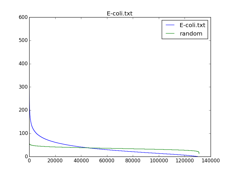
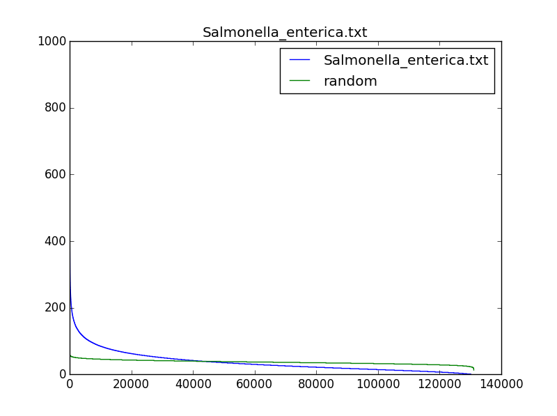
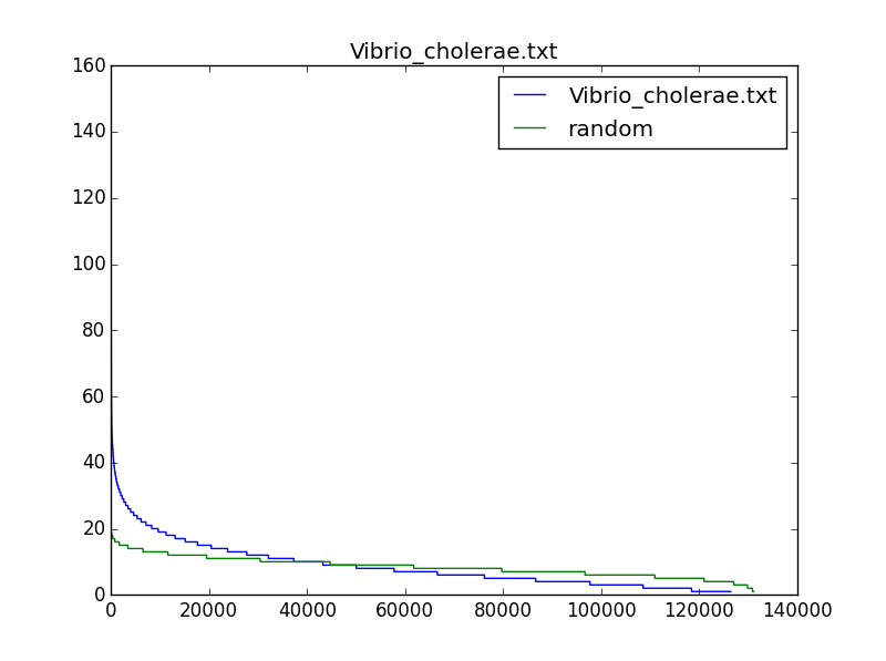
We may be able to find biologically interesting 9-mers if we search for (500,4)-clumps, and we will certainly identify fewer strings. However, these 9-mers might have nothing to do with DnaA boxes and ori regions because many ori regions have fewer than four DnaA boxes. Nevertheless, it is interesting to examine whether the most "clumped" regions in a bacterial genome reveal biologically interesting k-mers.

In this detour, we approximate the probability Pr(N, A, Pattern, t) that a string Pattern appears t or more times in a random string of length N formed from an alphabet of A letters. We prove that Pr(4, 2, "01", 1) = 11/16 by showing that 11 out of 16 binary strings of length 4 contain the string "01". The detour also describes the approximation

where C(·, ·) the combination statistic, n is defined as N-t·k, and k is the length of Pattern). For Pr(4, 2, "01", 1), n = 4 - 1 · 2 = 2 and this approximation results in

which is slightly higher than the correct probability 11/16. The "over-counting" happened because the described approximation counts some strings contributing to Pr(4, 2, "01", 1) more than once. Indeed, the approximation assumes that "01" may appear at any of three possible positions in a random string of length 4 as shown below ("?" refers to 0 or 1):

Since there are two possibilities for each "?" in the strings above (0 or 1), we end up with 3·4 = 12 strings:

However, we counted the boldfaced string "0101" twice.

For this question, we do not feel the need to reinvent the wheel. One of our former students found an excellent YouTube video illustrating these details.

Indeed, the scoring function in the Frequent Words with Mismatches and Reverse Complements Problem may count the same k-mers twice if these k-mers contributes to both Count_d(Text, Pattern) and Count_d(Text, ReverseComplement(Pattern)). For example, CTTCAG and its reverse complement CTGAAG are very similar, and both are just one mismatch away from Text = CTGCAG. Thus, Count₁(Text, CTTCAG) and Count₁(Text, CTTCAG) will both count an approximate occurrence of CTGCAG twice. Thus, to improve our scoring function, the first thing that comes to mind is to divide Count_d(Text, Pattern) + Count_d(Text, Pattern) by 2 for a string Pattern that is a reverse palindrome (i.e., the reverse complement of Pattern is itself).

However, it becomes less clear what to do if Pattern is almost equal to its reverse complement. For the sake of simplicity, we are therefore willing to close our eyes to the limitations on our scoring function posed by reverse palindromes. However, we should be wary of any candidates for DnaA boxes that are reverse palindromes (or nearly reverse palindromes).

Let's walk through deamination as it applies to a segment of double-stranded DNA. In the top of the figure below, the replication fork is about to open the seven base pairs shown and start replicating them. The (forward) half-strand on top is being synthesized as a single piece, whereas the (reverse) half-strand on the bottom is being synthesized in Okazaki fragments. The bottom strand is more vulnerable to deamination because it spends more time single-stranded than the top strand. The process of deamination is shown on the bottom in the figure below.

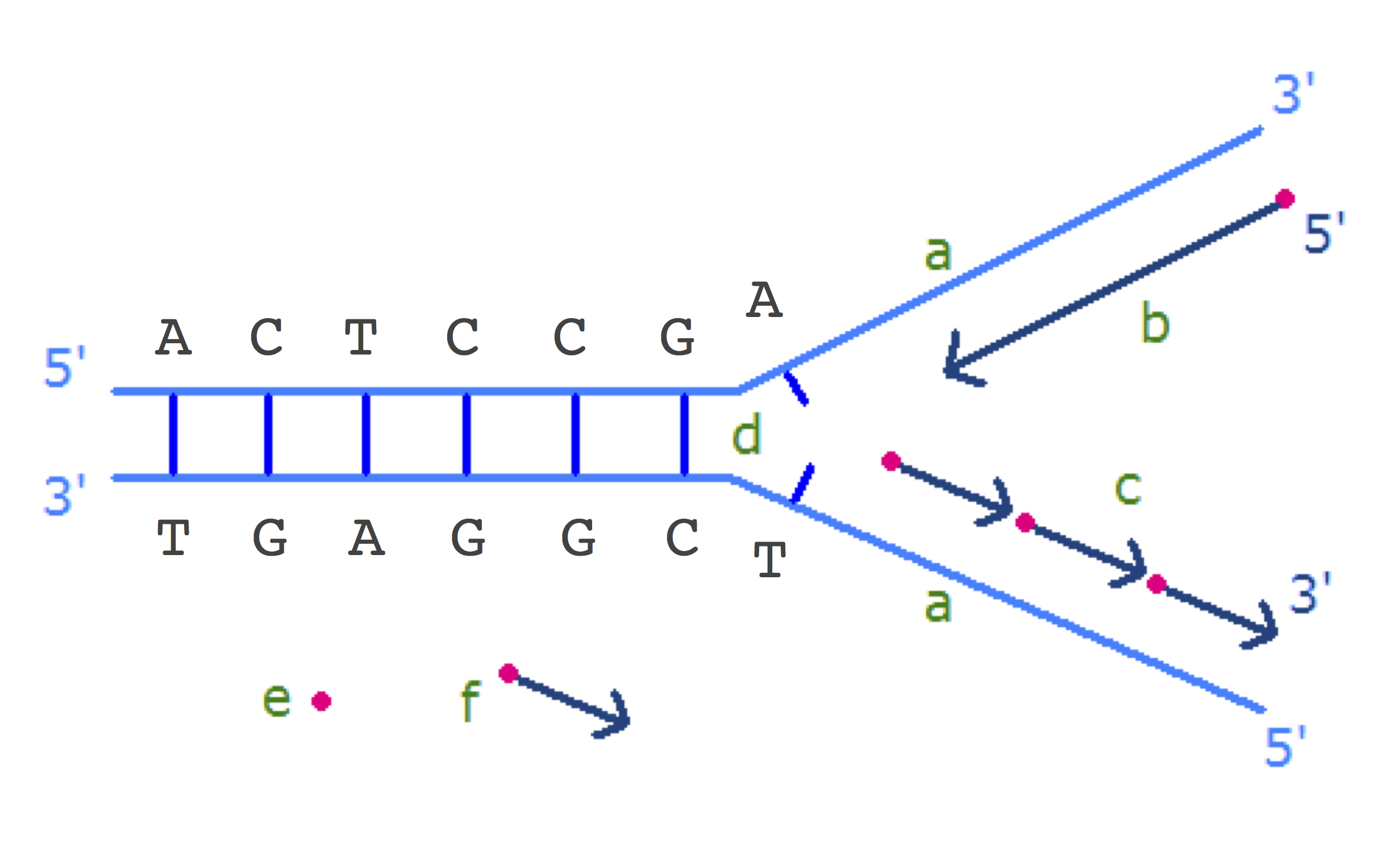
Figure: (Top) A replication fork is about to open seven base pairs. (Bottom) Deamination leads to a mutation of C into T and occurs on the bottom strand, where Okazaki fragments are being synthesized. Since the strand on the top is synthesized all at once, it has much smaller chance to be deaminated. After replication finishes, there are the two daughter strands, one of them with a mutation. The arrows indicate the direction of strand synthesis.

A set of supplemental slides attempting to further explain this can be found at this link.

At the beginning of the genome, the skew is set equal to zero. At the end of the genome, the skew should be equal to the total number of G's minus the total number of C's encountered in the genome. So this value will only equal zero if the genome has equal amounts of cytosine and guanine, which is unlikely.

Either of these two alternatives is perfectly reasonable. But computing the skew as the difference between G and C performed the best in practice.

In particular, you may have noticed that the frequency of T on the forward half-strand hardly changed. Although deamination initially creates a surplus of thymine on the forward half-strand, this surplus may be reduced by follow-up mutations of thymine into other nucleotides. In fact, deamination is just one of many factors that may contribute to skew. See Frank and Lobry, 1999 for a review of various mechanisms that contribute to the GC-skew. Tillier and Collins, 2000 even argued that deamination is not the major factor contributing to GC-skew. The question is whether there is some mechanism that makes GC-skew such a useful tool for identifying the location of ori in some species (like E. coli) but not others.

Because the vast majority of a bacterium’s genome serves a vital purpose in its survival, only a small fraction of cytosine can be mutated and maintain a viable bacterium.

The skew diagram is constructed by walking along the strand of DNA in the 5’ → 3’ direction (see figure reproduced below). Therefore, the skew diagram constructed for the complementary strand of E. coli will change, since we will be traversing the genome in the opposite direction.

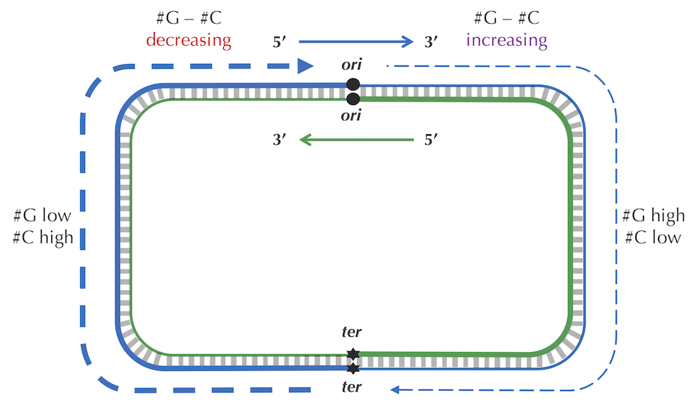
For example, if the E. coli skew diagram (reproduced below) is obtained by traversing the genome starting from some position in the genome above in the clockwise direction, then the skew diagram constructed for another strand corresponds to traversing the genome starting from the same position but in the counterclockwise direction.

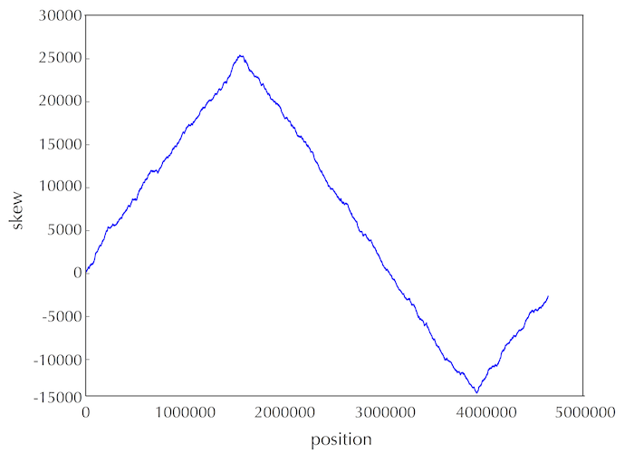
Also, note that for every interval of DNA, the difference between the amount of cytosine and guanine on the two strands have the same absolute values but different signs. Thus, the skew histogram for one strand is the "reversal" of the skew diagram for another strand. However, the minimum in both skew diagrams point to the same position in the genome.

If you look at a double-stranded genome, then the number of occurrences of G and C are the same because guanine pairs with cytosine (we do not account for the rare cases of mismatched base pairs caused by damage to DNA). However, the number of occurrences of G and C within a single strand may differ substantially.

Furthermore, despite base pairing, the amount of guanine and cytosine may be very different than the amount of adenine and thymine. For this reason, biologists refer to the percentage of guanine and cytosine nucleotides in a genome as the genome's GC-content. GC-content varies between species; the GC-content of the bacterium Streptomyces coelicolor is 72%, whereas the GC-content of the pathogen Plasmodium falciparum, which causes malaria, is only about 20%. In humans, the GC-content is about 42%.

Although there are no rigorous guidelines for selecting the parameter d in practice, biologists usually follow their intuition. On the one hand, d should not be too small, or else we may miss the biologically correct frequent word; on the other hand, d should not be too large, since many spurious approximate matches might be classified as putative DnaA boxes. In practice, biologists also analyze variations in experimentally confirmed DnaA boxes from well-studied bacteria and derive statistics for the expected number of mutations from the "canonical" DnaA box. It turns out that most of these studies identify canonical DnaA boxes that are very conserved, having no more than one or two mutations.

An insertion or deletion would likely prevent DnaA from being able to bind to the DnaA box because the interval is so short.

This was an arbitrary choice, and we got lucky this time. In practice, biologists should explore various windows in the vicinity of the minimum skew.

E. coli indeed contains ten 23 base pair hidden messages that are responsible for terminating replication. These messages are binding sites for the Tus protein, which works as a replication fork trap. Each Tus binding site is asymmetric, meaning that it will halt the replication fork moving in one direction and allow the other replication fork to proceed until it is stopped by its own fork trap. Can you find all ten Tus binding sites in E. coli without knowing what they are in advance?

ComputingFrequencies can be made more memory-efficient using hashing. However, implementing a hash table from scratch is more difficult than implementing a frequency array. In some languages like Python or Go, hash tables are built-in and not difficult to implement, we want our book to be language-blind so that students who program in any language can easily implement its algorithms.

Estimating the running time of recursive algorithms can be tricky – you might like to consult Wikipedia to learn about the "Master Theorem", which often helps us analyze the running time of recursive algorithms. However, the running time of Neighbors(Pattern, d) can be evaluated by noticing that this algorithm simply generates all d-neighborhoods of all suffixes of Pattern and computes the Hamming distance between each string in each d-neighborhood and the corresponding suffix. Thus, if we denote the size of the d-neighborhood of a pattern of length n as size_d(n), then the running time of Neighbors(Pattern, d) is:

If we use the notation sizeⁱ(n) to denote the number of strings having Hamming distance exactly i from any given string of length n, then

and the running time of Neighbors(Pattern, d) is

The only thing left is to compute sizeⁱ(n) for any values of i and n, which we leave to you as an exercise. :)