Lesson 5.13

Space Efficient Sequence Alignment

10 min read2 code challenges✓ Read

Watch the lectureSpace-Efficient Sequence Alignment

Computing alignment score using linear memory

To introduce fitting alignments, we used the example of aligning a 20,000 amino acid-long NRP synthetase from Bacillus brevis against a 600 amino acid-long A-domain from Streptomyces roseosporus. However, you may not be able to construct this alignment on your computer because the memory required to store the dynamic programming matrix is substantial.

The runtime of the dynamic programming algorithm for aligning two sequences of lengths n and m is proportional to the number of edges in their alignment graph, which is O(n · m). The memory required by this algorithm is also O(n · m), since we need to store the backtracking references. We will now demonstrate how to construct an alignment in just O(n) space at the expense of doubling the runtime (meaning that the runtime is still O(n · m)). In this section, for the sake of simplicity, we will consider the case of global alignment with non-affine gap penalties, i.e., when each symbol in a gap contributes the same score.

A divide-and-conquer algorithm often works when a solution to a large problem can be constructed from solutions of smaller problem instances. Such a strategy proceeds in two phases. The divide phase splits a problem instance into smaller instances and solves them; the conquer phase stitches the smaller solutions into a solution to the original problem. To learn more, see "DETOUR: Divide-and-Conquer Algorithms" in the print companion or at Cogniterra.

Before we proceed with the divide-and-conquer algorithm for linear-space alignment, note that if we only wish to compute the score of an alignment rather than the alignment itself, then the space required can easily be reduced to just twice the number of nodes in a single column of the alignment graph, or O(n). This reduction derives from the observation that the only values needed to compute the alignment scores in column j are the alignment scores in column j − 1. Therefore, the alignment scores in the columns before column j − 1 can be discarded when computing the alignment scores for column j, as illustrated in the figure below. Unfortunately, finding the longest path requires us to store an entire matrix of backtracking pointers, which causes the quadratic space requirement. The idea of the space reduction technique is that we don’t need to store any backtracking pointers if we are willing to spend a little more time. In fact, we will show how to construct an alignment without storing any backtracking pointers.

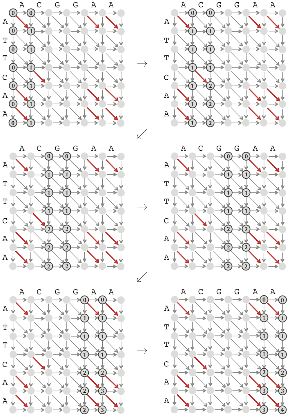
Figure: Computing an LCS alignment score by storing scores in just two columns of the alignment graph. As before,  all red edges have weight 1, and all other edges have weight 0.

The Middle Node Problem

Given strings v = v₁ ... v_n and w = w₁ ... w_m, define middle = \( \lfloor m/2 \rfloor \). The middle column of AlignmentGraph(v, w) is the column containing all nodes (i, middle) for 0 ≤ i ≤ n. A longest path from source to sink in the alignment graph must cross the middle column somewhere, and our first task is to figure out where using only O(n) memory. We refer to the node where the longest path crosses the middle column as a middle node (Note that different longest paths may have different middle nodes, and a given longest path may have more than one middle node.). In the figure below, middle = 3, and the optimal alignment path crosses the middle column at the (unique) middle node (4, 3).

The key observation is that we can find a longest path's middle node without having to construct this path in the alignment graph. We will classify a path from the source to the sink as an i-path if it passes through the middle column at row i. For example, the path highlighted below is a 4-path because it passes through the middle column at row 4. For each i between 0 and n, we would like to find the length of a longest i-path (denoted Length(i)) because the largest value of Length(i) over all i will reveal a middle node.

Exercise BreakFind all middle nodes for all longest paths when finding a longest common subsequence of ACCA and CAAC.

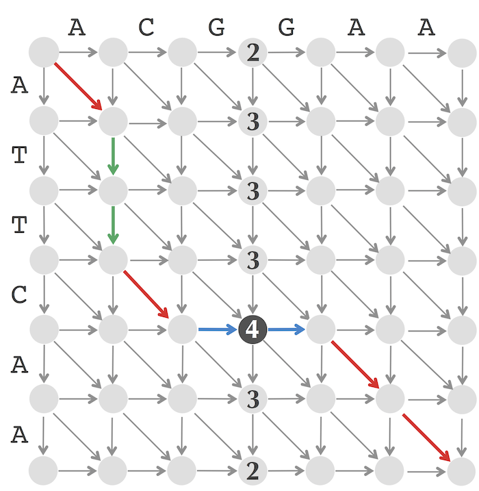
Figure: The alignment graph of ATTCAA and ACGGAA, with the LCS alignment path highlighted. The number inside each node (i, middle) in the middle column is equal to Length(i). The node maximizingLength(i) is a middle node (multiple middle nodes may exist); the middle node in this graph is colored black.

Let FromSource(i) denote the length of the longest path from the source ending at (i, middle) and ToSink(i) denote the length of the longest path from (i, middle) to the sink. Certainly,

Length(i) = FromSource(i) + ToSink(i),

and so we need to compute FromSource(i) and ToSink(i) for each i.

STOP and Think Can you compute FromSource(i) and ToSink(i) in linear space? How much time would it take?

The value of FromSource(i) is simply s_{i, middle} , which we already know can be computed in linear space. Thus, the values FromSource(i) for all i are stored as s_{i, middle} in the middle column of the alignment graph, and computing them requires sweeping through half of the alignment graph from column 0 to the middle column. Since we need to explore roughly half the edges of the alignment graph to compute FromSource(i), we say that the runtime needed for computing all values FromSource(i) is proportional to half of the “area” of the alignment graph, or n · m/2 (see figure below).

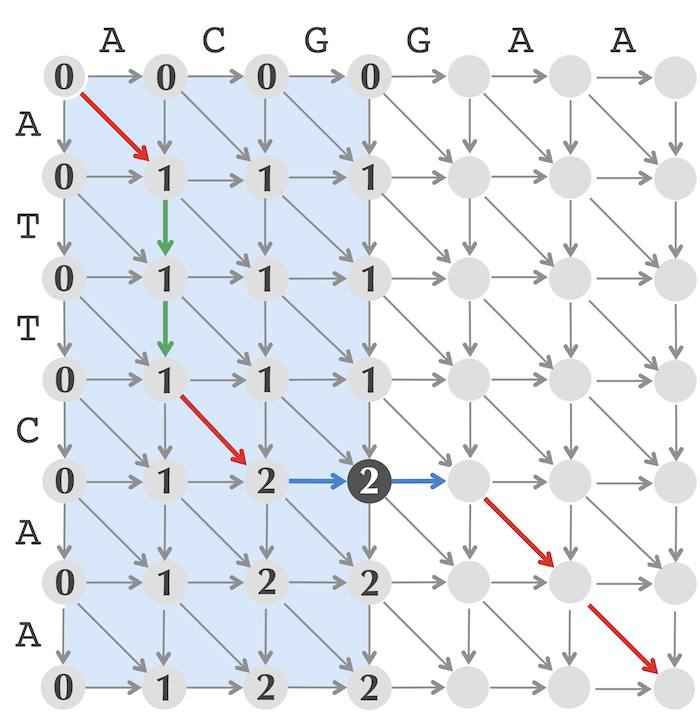
Figure: Computing FromSource(i) for all i can be done in O(n) space and time proportional to n · m/2.

Computing ToSink(i) is equivalent to finding the longest path from the sink to (i, middle) if all the edge directions are reversed. Instead of reversing the edges, we can reverse the strings v = v₁ ... v_n and w = w₁ ... w_m and find s_{n-i,m - middle} in the alignment graph for v_n ... v₁ and w_m ... w₁. Computing ToSink(i) is therefore similar to computing FromSource(i) and can also be done in O(n) space and runtime proportional to n · m/2 , or half of the area of the alignment graph (see figure below). In total, we can compute all values Length(i) = FromSource(i) + ToSink(i) in linear space with runtime proportional to n · m/2 + n · m/2 = n · m, which is the total area of the alignment graph.

It looks like we have wasted a lot of time just to find a single node on the alignment path! You may think that this approach is doomed to fail because we have already spent O(n · m) time (the entire area of the alignment graph) to gain very little information.

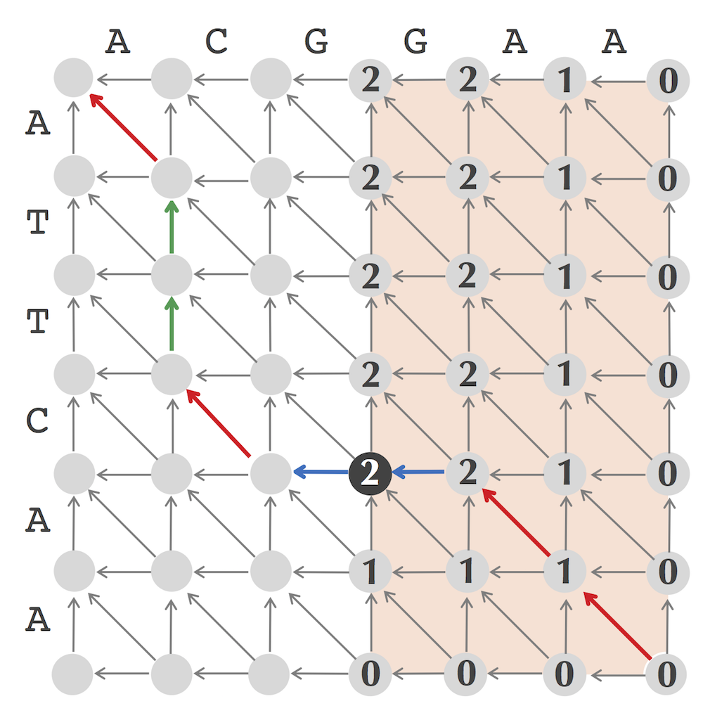
Figure: Computing ToSink(i) for all i can also be done in O(n) space and time proportional to n · m/2; this requires reversing the direction of all edges and treating the sink as the source.

A surprisingly fast and memory-efficient alignment algorithm

Once we have found a middle node, we automatically know two rectangles through which a longest path must travel on either side of the middle node. As shown in the figure below, one of these rectangles consists of all nodes above and to the left of the middle node, whereas the other rectangle consists of all nodes below and to the right of the middle node. Thus, the area of the two highlighted rectangles is half the total area of the alignment graph.

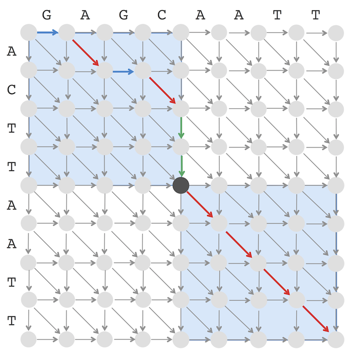
Figure: A middle node (shown in black) defines two highlighted rectangles and illustrates that the optimal path must travel within these rectangles. We can therefore eliminate the remaining parts of the alignment graph from consideration for an optimal alignment path.

We can now divide the problem of finding the longest path from (0, 0) to (n, m) into two subproblems: finding the longest path from (0,0) to the middle node; and finding the longest path from the middle node to (n, m). The conquer step finds the two middle nodes within the smaller rectangles, which can be done in time proportional to the sum of the areas of these rectangles, or n · m/2 (figure below). Note that we have now reconstructed three nodes of an optimal path.

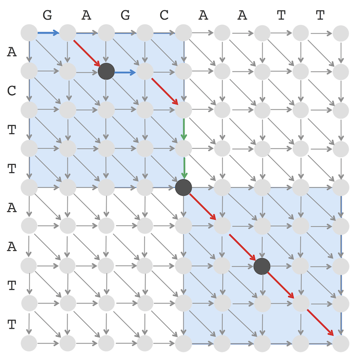
Figure: Finding middle nodes (shown as two more black circles) within the previously identified rectangles.

In the next iteration, we will divide and conquer to find four middle nodes in time equal to the sum of the areas of the even smaller blue rectangles, which have total area n · m/4 (see figure below). We have now reconstructed nearly all nodes of an optimal alignment path!

STOP and Think How much time would it take to find all nodes on an optimal alignment path?

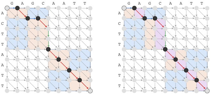
Figure: Finding middle nodes (highlighted as black circles) within previously identified blue rectangles.

In general, at each new step before the final step, we double the number of middle nodes found while halving the runtime required to find middle nodes. Proceeding in this way, we will find the middle nodes of all rectangles (and thus construct the entire alignment!) in time equal to

n·m + n·m/2 + n·m/4 + ··· < 2·n·m = O(n·m).

Thus, we have arrived at a quadratic-time algorithm that requires only linear space.

The Middle Edge Problem

Instead of asking you to implement a divide-and conquer algorithm based on finding a middle node, we will use a more elegant approach based on finding a middle edge, or an edge in an optimal alignment path starting at the middle node (more than one middle edge may exist for a given middle node). Once we find the middle edge, we again know two rectangles through which the longest path must travel on either side of the middle edge. But now these two rectangles take up even less than half of the area of the alignment graph (see figure below), which is an advantage of selecting the middle edge instead of the middle node.

Middle Edge in Linear Space Problem: Find a middle edge in the alignment graph in linear space.

• Input: Two strings and a matrix score.
• Output: A middle edge in the alignment graph of these strings (where the edge lengths are defined by score).

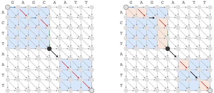
Figure: (Left) A middle edge (shown in bold) starts at a middle node (shown as a black circle). The optimal path travels inside the first highlighted rectangle, passes the middle edge, and travels inside the second highlighted rectangle afterwards. We can eliminate the remaining parts of the alignment graph, which takes up over half of the area formed by the graph, from further consideration. (Right) Finding middle edges (shown in bold) within previously identified rectangles.

Code Challenge Solve the Middle Edge in Linear Space Problem (for protein strings). Solve at Cogniterra or Rosalind.Solve it with the autograderFree to start in the interactive text

• Input: Two amino acid strings.
• Output: A middle edge in the alignment graph in the form "(i, j) (k, l)", where (i, j) connects to (k, l).

The pseudocode below for LinearSpaceAlignment describes how to recursively find a longest path in the alignment graph constructed for a substring v_top+1 ... v_bottom of v and a substring w_left+1 ... w_right of w. LinearSpaceAlignment calls the function MiddleNode(top, bottom, left, right), which returns the coordinate i of the middle node (i, j) defined by the sequences v_top+1 ... v_bottom and w_left+1 ... w_right. LinearSpaceAlignment also calls MiddleEdge(top, bottom, left, right), which returns → , ↓, or ↘ depending on whether the middle edge is horizontal, vertical, or diagonal. The linear-space alignment of strings v and w is constructed by calling LinearSpaceAlignment(0, n, 0, m). The case left = right describes the alignment of an empty string against the string v_top+1 ... v_bottom, which is trivially computed as the score of a gap formed by bottom − top vertical edges.

LinearSpaceAlignment(v, w, top, bottom, left, right)
  if left = right
    output path formed by bottom − top vertical edges
  if top = bottom
    output path formed by right − left horizontal edges
  middle ← ⌊ (left + right)/2⌋
  midEdge ← MiddleEdge(v, w, top, bottom, left, right)
  midNode ← vertical coordinate of the initial node of midEdge
  LinearSpaceAlignment(v, w, top, midNode, left, middle)
  output midEdge
  if midEdge = "→" or midEdge = "↘"
    middle ← middle + 1
  if midEdge = "↓" or midEdge ="↘"
    midNode ← midNode + 1
  LinearSpaceAlignment(v, w, midNode, bottom, middle, right)

One straightforward way to implement LinearSpaceAlignment is to output each edge as a symbol V (vertical), H (horizontal), or D (diagonal). The resulting string constructed from the 3-symbol alphabet {V, D, H} defines a path through the alignment graph and allows us to reconstruct the alignment.

Code Challenge Implement LinearSpaceAlignment to solve the Global Alignment Problem for a large dataset. Solve at Cogniterra or Rosalind.Solve it with the autograderFree to start in the interactive text

• Input: Two long (10000 amino acid) protein strings written in the single-letter amino acid alphabet.
• Output:The maximum alignment score of these strings, followed by an alignment achieving this maximum score.

Exercise Break: Design a space-efficient algorithm for local sequence alignment.