Lesson 2.3
Scoring Motifs
Watch the lectureFrom Implanted Patterns to Regulatory Motifs (Part 2)
From motifs to profile matrices and consensus strings
Although the Implanted Motif Problem offers a useful abstraction of the biological problem of motif finding, it has some limitations. For example, when Steve Kay used a DNA array to infer the set of circadian genes in plants, he did not expect that all genes in the resulting set would have the evening element (or its variants) in their upstream regions. Similarly, biologists do not expect that all genes with an elevated expression level in infected flies must be regulated by NF-κB. DNA array experiments are inherently noisy, and some genes identified by these experiments have nothing to do with the circadian clock in plants or immunity genes in flies. For such noisy datasets, any algorithm for the Implanted Motif Problem would fail, because as long as a single sequence does not contain the transcription factor binding site, a (k, d)-motif does not exist!
A more appropriate problem formulation would score individual instances of motifs depending on how similar they are to an “ideal” motif (i.e., a transcription factor binding site that binds the best to the transcription factor). However, since the ideal motif is unknown, we attempt to select a k-mer from each string and score these k-mers depending on how similar they are to each other.
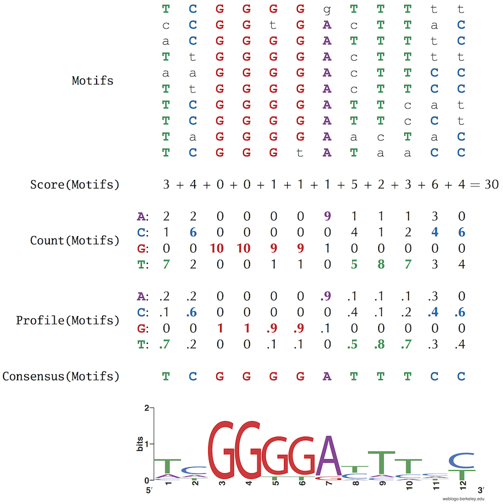
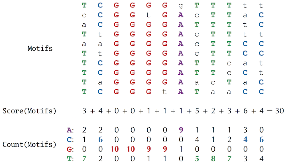
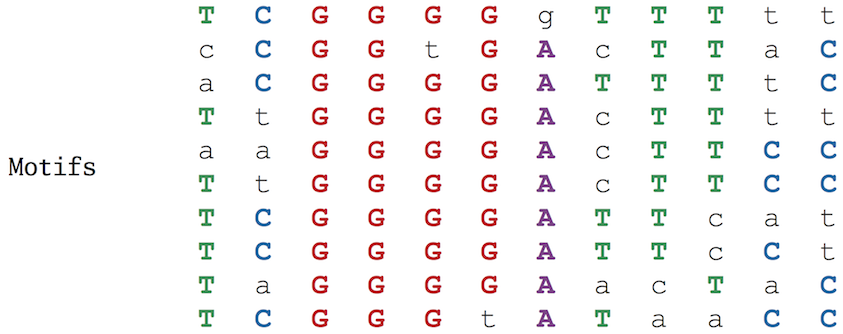
To define scoring, consider a list of t DNA strings Dna, where each string has length n, and select a k-mer from each string to form a collection Motifs, which we represent as a t x k motif matrix. In the figure below, which shows the motif matrix for the NF-κB binding sites from the figure below, we indicate the most frequent nucleotide in each column of the motif matrix by upper case letters. If there are multiple most frequent nucleotides in a column, then we arbitrarily select one of them to break the tie. Note that positions 2 and 3 are the most conserved (nucleotide G is completely conserved in these positions), whereas position 10 is the least conserved.
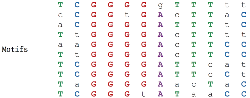
Figure: The NF-κB binding sites form a 10 x 12 motif matrix, with the most frequent nucleotide in each column shown in upper case letters and all other nucleotides shown in lower case letters.
By varying the choice of k-mers in each sequence, we can construct a large number of different motif matrices from a given sample of DNA sequences. Our goal is to select k-mers resulting in the most “conserved” motif matrix, meaning the matrix with the most upper case letters (and thus the fewest number of lower case letters). Leaving aside the question of how we select such k-mers, we will first focus on how to score the resulting motif matrices, defining Score(Motifs) as the number of unpopular (lower case) letters in the motif matrix Motifs. Our goal is to find a collection of k-mers that minimizes this score.
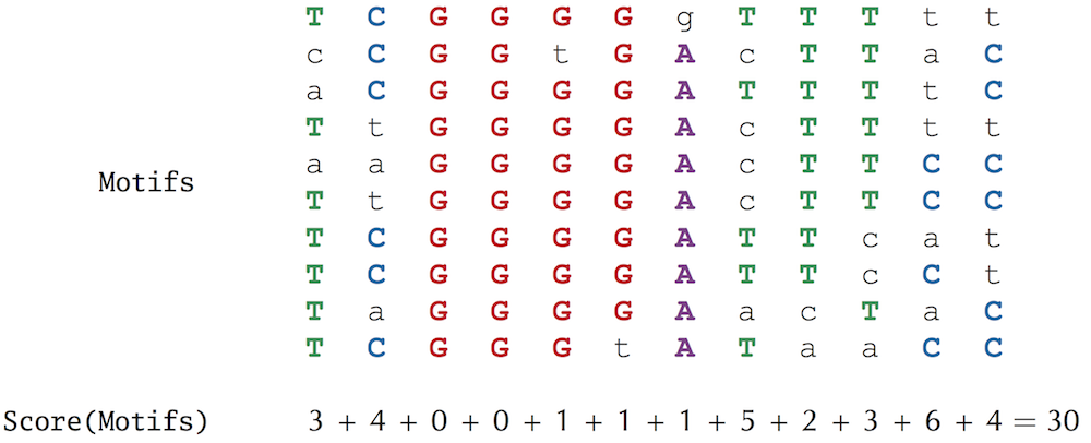
Exercise Break The minimium possible value of Score(Motifs) is 0 (if all the k-mers in Motifs are the same). What is the maximum possible value of Score(Motifs) for 10 motifs of length 15?
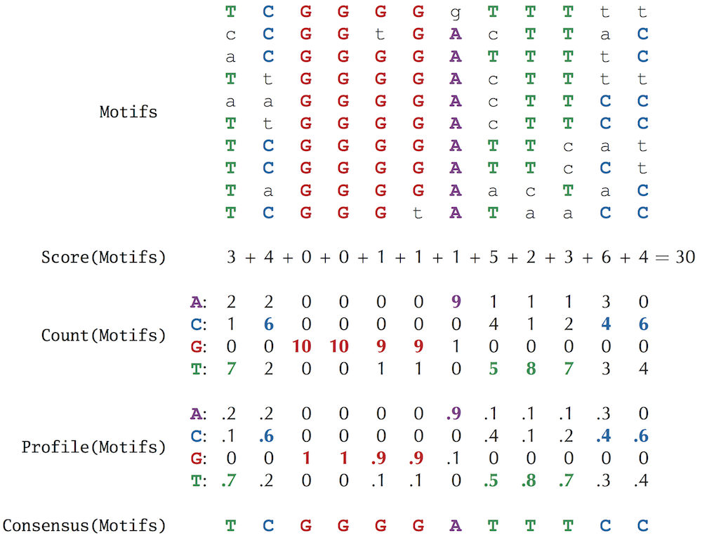
We can construct the 4 × k count matrix Count(Motifs) counting the number of occurrences of each nucleotide in each column of the motif matrix; the (i, j)-th element of Count(Motifs) stores the number of times that nucleotide i appears in column j of Motifs. We will further divide all of the elements in the count matrix by t, the number of rows in Motifs. This results in a profile matrix P = Profile(Motifs) for which Pi,j is the frequency of the i-th nucleotide in the j-th column of the motif matrix. Note that the elements of any column of the profile matrix sum to 1. The figure below shows the motif, count, and profile matrices for the NF-κB binding sites.

Finally, we form a consensus string, denoted Consensus(Motifs), from the most popular letters in each column of the motif matrix. If we select Motifs correctly from the collection of upstream regions, then Consensus(Motifs) provides an ideal candidate regulatory motif for these regions. For example, the consensus string for the NF-κB binding sites in the figure below is TCGGGGATTTCC.
Towards a more adequate motif scoring function
Consider the second column (containing 6 C, 2 A, and 2 T) and the final column (containing 6 C and 4 T) in the motif matrix reproduced below. Both of these columns contribute 4 to Score(Motifs).
STOP and Think Does scoring these two columns equally make sense biologically?
For many biological motifs, certain positions feature two nucleotides with roughly the same ability to bind to a transcription factor. For example, the sixteen nucleotide-long CSRE transcription factor binding site in the yeast species S. cerevisiae consists of five strongly conserved positions (1, 8, 9, 12, and 13) in addition to eleven weakly conserved positions, each of which features two nucleotides with similar frequencies (see figure below).

Following this example, a more appropriate representation of the consensus string TCGGGGATTTCC for the NF-κB binding sites should include viable alternatives to the most popular nucleotides in each column. For example, nucleotides with frequencies equal to or exceeding 0.4. In this sense, the last column (6 C, 4 T) in the NF-κB motif matrix (reproduced below) is “more conserved” than the 2nd column (6 C, 2 A, 2 T) and should receive a lower score.
Entropy and the motif logo
Every column of Profile(Motifs) corresponds to a probability distribution, or a collection of nonnegative numbers that sum to 1. For example, the 2nd column in the profile matrix for the NF-κB binding sites corresponds to the probabilities 0.2, 0.6, 0.0, and 0.2 for A, C, G, and T, respectively.

Entropy is a measure of the uncertainty of a probability distribution (p1, …, pN), and is defined as follows:
H(p1, ... pN) = -Σi=1N pi · log2 pi
For example, the entropy of the probability distribution (0.2, 0.6, 0.0, 0.2) corresponding to the 2nd column of the NF-κB profile matrix is
-(0.2 log2 (0.2) + 0.6 log2 (0.6) + 0.0 log2 (0.0) + 0.2 log2 (0.2) ≈ 1.371
whereas the entropy of the more conserved final column (0.0, 0.6, 0.0, 0.4) is
-(0.0 log2 (0.0) + 0.6 log2 (0.6) + 0.0 log2 (0.0) + 0.4 log2 (0.4)) ≈ 0.971
and the entropy of the very conserved 5th column (0.0, 0.0, 0.9, 0.1) is
-(0.0 log2 (0.0) + 0.0 log2 (0.0) + 0.9 log2 (0.9) + 0.1 log2 (0.1) ) ≈ 0.467
Note: Technically, log2(0) is undefined, but in the computation of entropy, we assume that 0 · log2(0) is equal to 0.STOP and Think What are the maximum and minimum possible values for the entropy of a probability distribution containing four values?
The entropy of the completely conserved third column is 0, which is the minimum possible entropy. On the other hand, a column with equally-likely nucleotides (all probabilities equal to 1/4) has maximum possible entropy −4 · 1/4 · log2(1/4) = 2. In general, the more conserved the column, the smaller its entropy. Thus, entropy offers an improved method of scoring motif matrices: the entropy of a motif matrix is defined as the sum of the entropies of its columns. In this book, we will continue to use Score(Motifs) for simplicity, but the entropy score is used more often in practice.
Exercise Break Compute the entropy of the NF-κB motif matrix (reproduced below).
Another application of entropy is the motif logo, a diagram for visualizing motif conservation that consists of a stack of letters at each position. We show a motif logo for the NF-κB motif matrix at the bottom. The relative sizes of letters indicate their frequency in the column. The total height of the letters in a column is based on the information content of the column, which is defined as 2 − H(p1, … , pN). The lower the entropy, the higher the information content, meaning that tall columns in the motif logo are highly conserved.